
 hesperia [dot] info [at] hesperia-space [dot] eu
To run this software, the user needs to consider two main blocks. The first one concerns the storage of the data needed for the GLE inversion. This includes NM data, the computed asymptotic directions of the NM stations, the OMNI magnetic field data in GSE coordinates and a database of results of an interplanetary transport model. The second block requires these data to invert the problem and infer from the measured NM relative increases the characteristics of the solar source (injection profile and spectral index) and the interplanetary transport conditions.
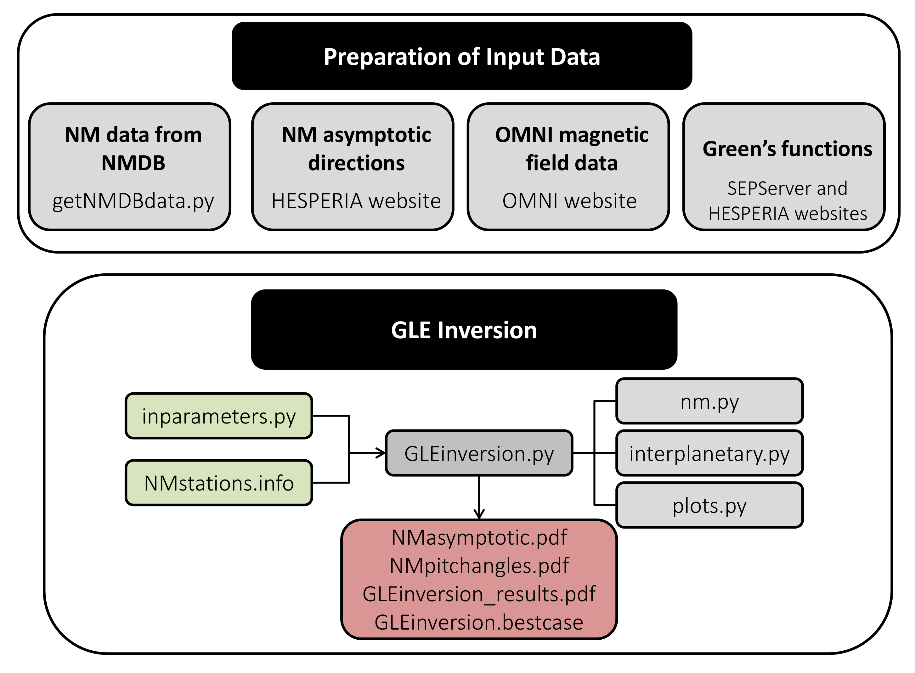
Preparation of Input Data
- Run the program getNMDBdata.py to directly download 5-min NM data from the Neutron Monitor Data Base (NMDB) to the user’s computer by using the NMDB Nest tool. The time interval, i.e. start and end time, during which the NM data should be downloaded has to be given in the first lines of the program code.
- Download the computation results of the cosmic ray particle trajectories in the geomagnetic field, i.e. the asymptotic directions of the NM stations for the selected time of the GLE under investigation. Download them from here. It is required that the asymptotic directions are in Geocentric Solar Ecliptic (GSE) coordinates. In principle, users of the GLE inversion software are free to determine the asymptotic directions for the selected NM stations and for the selected date and time by using e.g. different models for the Earth's magnetic field. That goes without saying that the self generated files must have the same format.
- Download annual 5-min OMNI interplanetary magnetic field data in GSE coordinates from the OMNI database. The OMNI database provides a well-documented dataset of time-shifted magnetic field observations, which describe the field evolution at the nose of the Earth’s bow shock as a function of time. The GLE inversion software uses the magnetic field vector to compute the pitch angles observed by each NM station, i.e. the angle between the magnetic field direction and the asymptotic directions of each NM station. The interplanetary magnetic field data is averaged over a 30 min time window.
- Download the Green’s functions of the interplanetary transport, which are the results of an interplanetary transport model that simulates the propagation of relativistic solar energetic particles along the interplanetary magnetic field. Adiabatic deceleration in the interplanetary space as well as effects of diffusion perpendicular to the average magnetic field and drifts are neglected in the interplanetary transport model. In addition, it is assumed that there is no variation across the magnetic field and that respective solutions are identical in neighboring flux tubes. One of the limitations of this database is, that it is not useful for the study of particle events showing bidirectional pitch-angle distributions. The database of Green’s functions is available in SEPServer and in the HESPERIA website.
GLE Inversion
The GLE inversion software consists of 6 files:
- GLEinversion.py: This is the main program. To run the GLE inversion program the user needs to type python GLEinversion.py in the terminal.
- nm.py: It is a module required by the main program. It contains functions to read NM data and the asymptotic direction files, and to compute the simulated relative NM count rate increases.
- interplanetary.py: It is a module required by the main program. It contains functions to read the Green's functions of interplanetary transport, the OMNI magnetic field and handle its averaging, and perform the inversion of the problem.
- plots.py: It is a module required by the main program. It contains functions to plot the results determined by the software.
- inparameters.py: It is the file with the input parameters used by the software where the user needs to specify:
- the beginning and end of the fitting period (Note it is limited to 3 h),
- the start and end time of the baseline interval, i.e. a time interval before the GLE to determine the count rate caused by the actual galactic cosmic ray intensity, usually the full hour before the onset of the GLE is used,
- where in his/her computer the relevant data is stored. This includes: directory where the NM data files are located, the directory with computed NM asymptotic directions, the directory with the 5-min OMNI magnetic field data, the directory with the Green’s functions of interplanetary transport,
- the interplanetary magnetic field polarity (+1 or -1). The IMF polarity can be inferred by inspecting the pitch-angle distributions of suprathermal electrons measured by e.g. ACE. These plots also provide information about whether the Earth is in an open/closed field line configuration,
- the range of values of the proton mean free path at rigidity 2 GV (λ0) that the user would like to test. Note that the software can properly handle values between 0.05 and 0.9 AU only,
- the range of values of the spectral index of the solar source spectrum (dN/dR = R-γ) that the user would like to test.
- NMstation.info: This ASCII file contains relevant information about each NM station such as: NM short name, NM full name, geographic latitude and longitude of the NM station, altitude of the NM station, reference pressure of the NM station, barometric coefficient of the NM station, number of counter tubes and cutoff rigidity of the NM station.
In addition, the GLE inversion software makes use of the following Python libraries and modules: numpy, scipy, matplotlib, os, datetime and bisect.

